Fokker Planck equation
Description
The Fokker Planck equation has the form
where
is a smooth function,
some parameter and
a probability density on
. The partial differential equation is in divergence form and conserves mass. Hence, also
is a probability density on
. In the case, where
has some growth at
, the equilibrium solutions
are characterized by
leading to the solution
The density
is called Gibbs distribution, which accounts to the fact, that it minimizes the (Gibbs) free energy
where
is the energy and
the (Gibbs-Boltzmann) entropy
By this formulation
plays the role of the inverse temperature. Note, that the Euler-Lagrange equation is given by
which is solved by .
Pathwise formulation via stochastic differential equations
The stochastic process
defined by
where is an -dimensional Brownian motion, is the pathwise formulation of the Fokker Planck equation. If distribution of the initial random vector is given by , then at later times the solution has distribution , where is solution of the Fokker Planck equation.
The dynamic of the pathwise formulation undergoing diffusion in the potential . The particle is solely described by its position , i.e. inertia is neglected. Then, the particle chooses the steepest descent with respect ot , which is perturbed by random fluctuation, which are assumed to be normal distributed. The coupling parameter describing the strength of the fluctuations plays again the role of inverse temperature. In particular, the limit describes the behaviour of the system without fluctuations.
Ornstein-Uhlenbeck process
A prominent example, which can be explicitly solved, is the Ornstein-Uhlenbeck process, corresponding to the choice
The stationary distribution is given by the Gaussian
The underlying picture becomes particular simple in one dimension. There, the leading order behaviour of the process can be characterized by its mean
and variance
, which are given by
Both,
and
, satisfy an ordinary differential equation not depending on
Hence, the mean converges exponentially fast to
with rate
and the variance converges exponentially fast from the initial variance
to
with rate
Numerical example
For general potentials explicit solutions of the Fokker Planck equation are not available. However, the pathwise formulation allows to do Monte-Carlo simulation of single realisations of the process . The case, where is not convex is especially interessting, because at low temperature, i.e. , the process shows metastable behaviour.
Therefore, we consider the potential function looking like
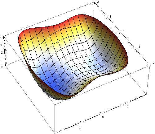
The realization of the process for increasing values of :
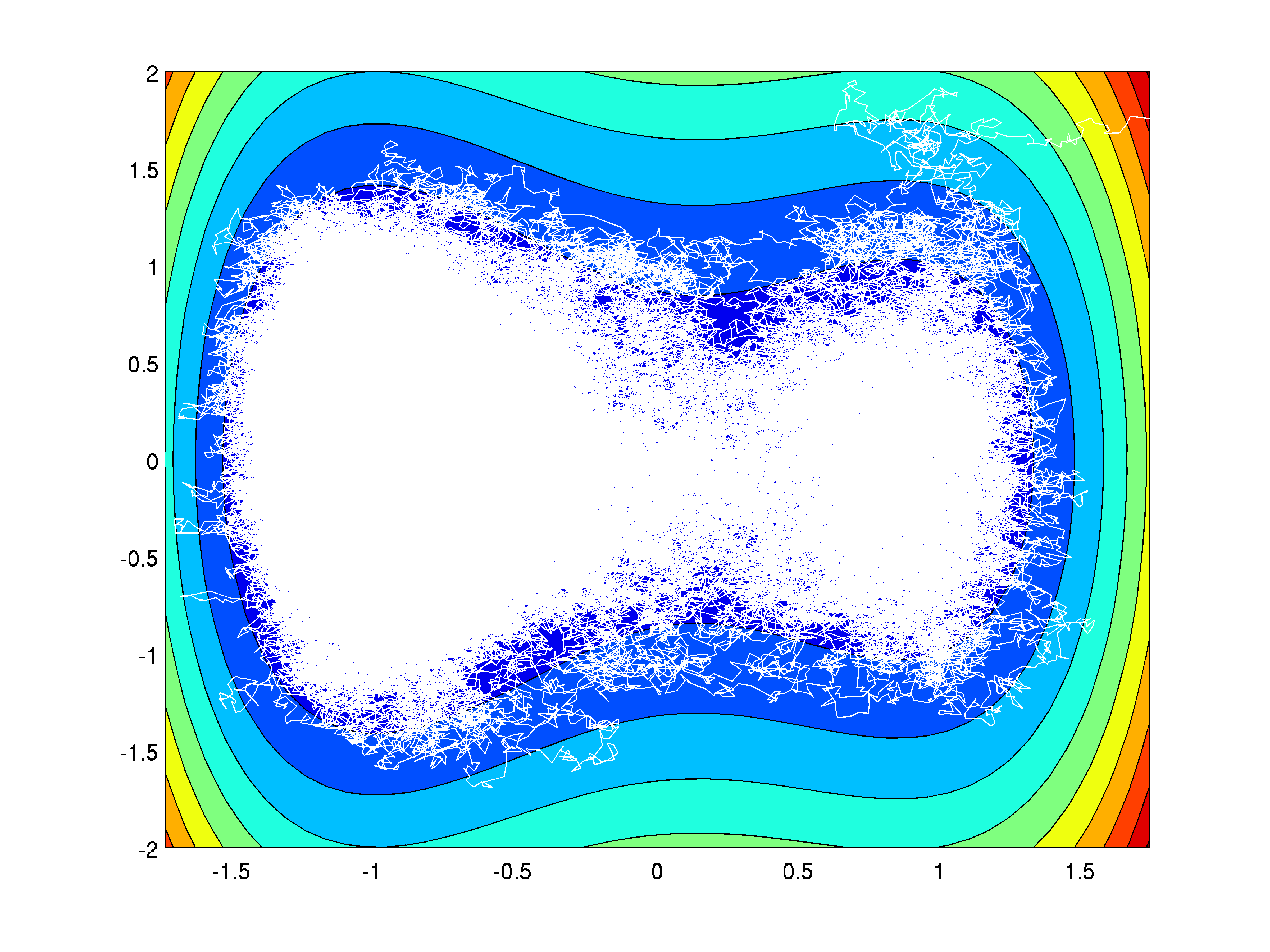
Monte Carlo simulation for Fokker Planck equation
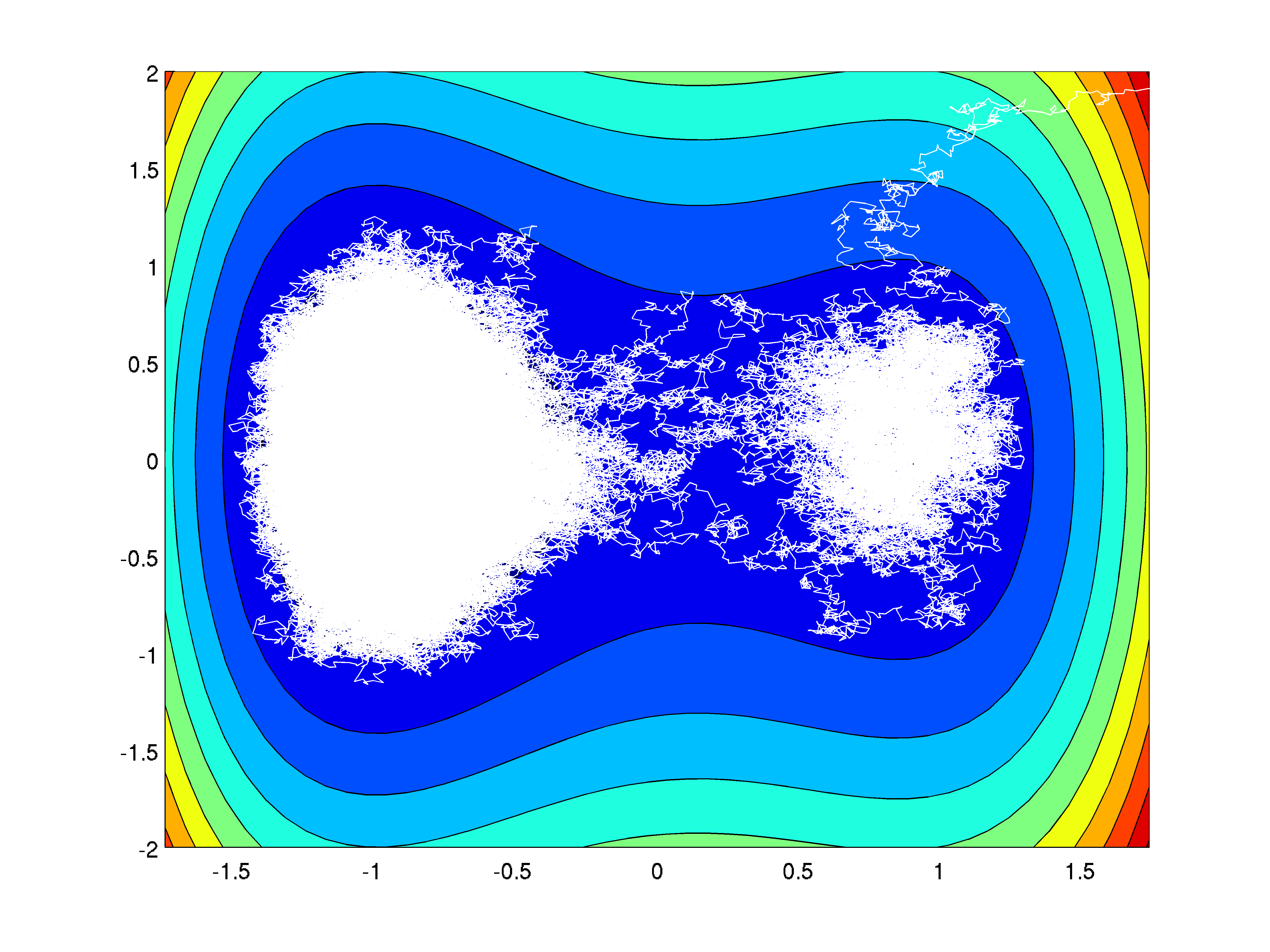
Monte Carlo simulation for Fokker Planck equation
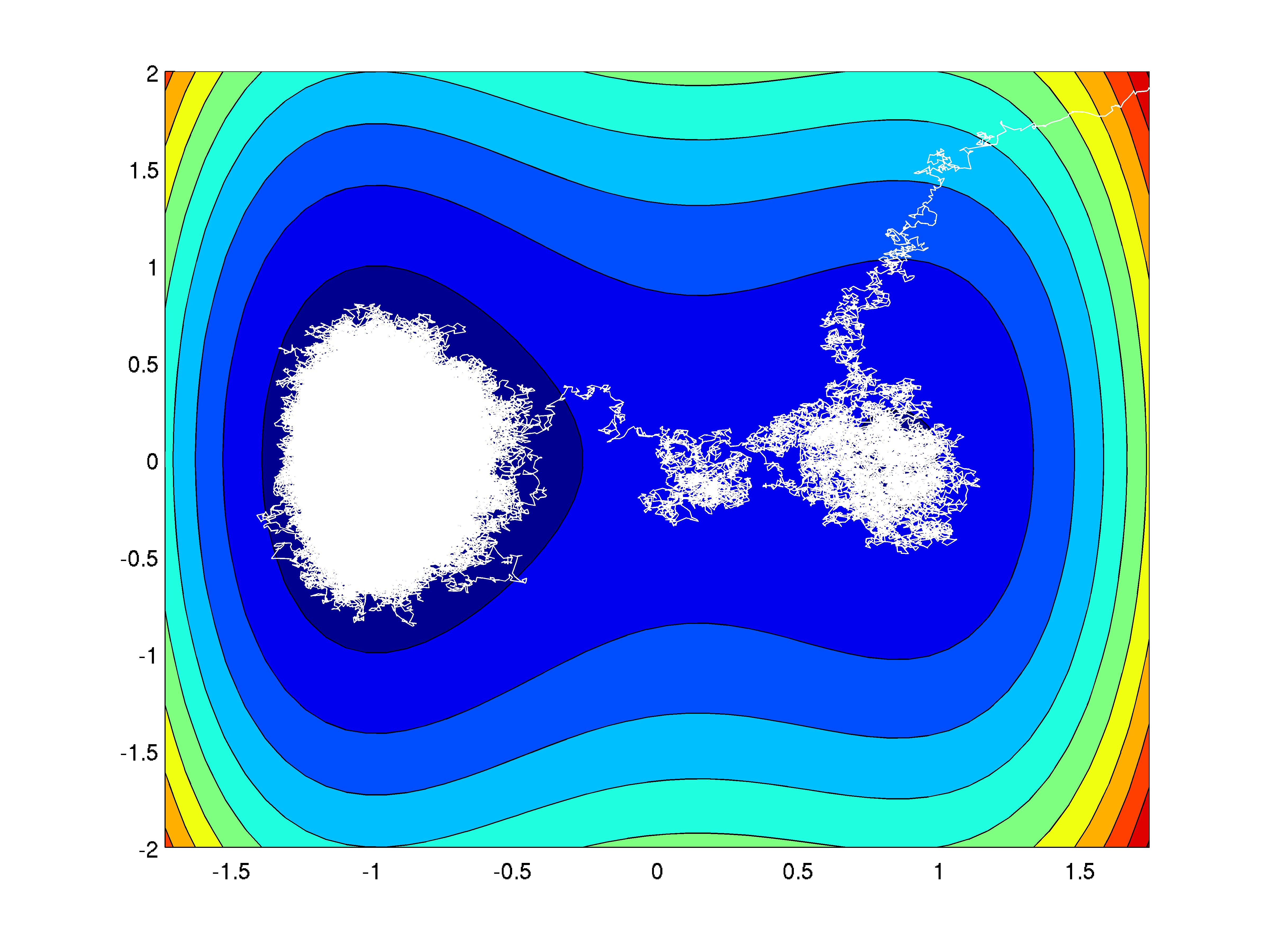
Monte Carlo simulation for Fokker Planck equation
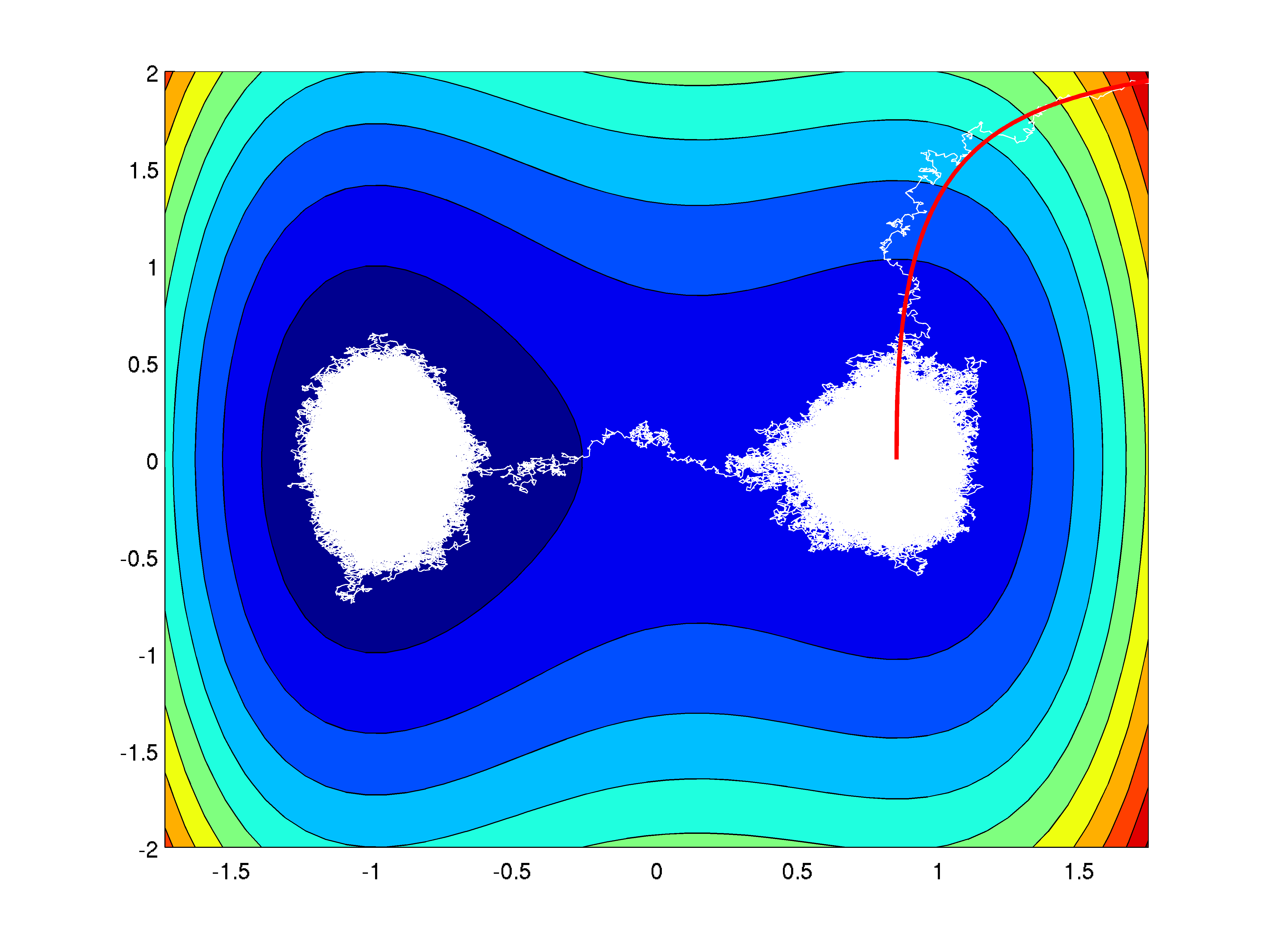
Monte Carlo simulation for Fokker Planck equation (red )
For increasing values of the particle goes quickly to the local minima and is trapped there longer and longer times. The transition to the global energy minimizing state happens along a path crossing the saddle. This behaviour is called metastable. For the limiting dynamic without any fluctuation a transition is not possible and the particle is stuck in the local minima.
References
- R. Jordan, D. Kinderlehrer, and F. Otto, “The Variational Formulation of the Fokker-Planck Equation,” SIAM Journal on Mathematical Analysis, vol. 29, no. 1, 1998.