Metastability

20 October 2015

Metastablity by decomposition of the potential

The project (together with Georg Menz) considers as a prime example a Fokker-Planck equation in a multi-well potential and calculates the precise rate of convergence to equilibrium. The convergence to equilibrium is measures in variance and in relative entropy. We consider the following parabolic PDE

\partial_t \varrho_t = \varepsilon \Delta \varrho_t + \nabla \cdot ( \varrho_t \nabla H ) ,

with invariant measure in Gibbs form $\mu(dx) = \exp(-H/\varepsilon)$ . Therewith, the generator is symmetric in $L^2(d\mu)$ . Therefor, it is convenient to consider the evolution of $f_t := \varrho_t / \mu$ . Then, for this evolution the variance and relative entropy defined by

\operatorname{var}_\mu(f) = \int (f - \bar f)^2 d\mu \quad\text{and}\quad \operatorname{Ent}_\mu(f) = \int f \log \frac{f}{\bar f} d\mu,

with $\bar f := \int f d\mu$ , are decresing in time:

\frac{d}{dt} \operatorname{var}(f_t) = - 2 \int |\nabla f|^2 d\mu \quad \text{and}\quad \frac{d}{dt} \operatorname{Ent}(f_t) = - \int \frac{|\nabla f|^2}{f} d\mu .

Exponential convergence to equilibrium is established by a simple Gronwall arguemnt, if one is able to connect the quantities on the right hand side back to the variance and relative entropy, respectively. The functional inequalities needed in this case are the Poincaré (PI( and the logarithmic Sobolev inequality

\operatorname{var}_\mu(f) \leq C_{\mathrm{PI}} \int |\nabla f|^2 d\mu \quad \text{and} \quad \operatorname{Ent}_\mu(f) \leq C_{\mathrm{Ent}} \int \frac{|\nabla f|^2}{f} d \mu .

The main result in

Georg Menz, André Schlichting. Poincaré and logarithmic Sobolev inequalities by decomposition of the energy landscape. Annals of Probability. Volume 42, Number 5 (2014), 1809-1884. [ link | arXiv | pdf ]

proves asymptotic estimates in $\varepsilon$ for the constants $C_{\mathrm{PI}}$ and $C_{\mathrm{Ent}}$ .

The main idea comes from the simple observation, that a sample path of the according SDE

dX_t = - \nabla H(X_t) dt + \sqrt{2\varepsilon} d B_t ,

with $B_t$ a standard Brownian motion in $\mathbb{R}^d$ . Then, a typical picture of a sufficiently long trajectories looks like:

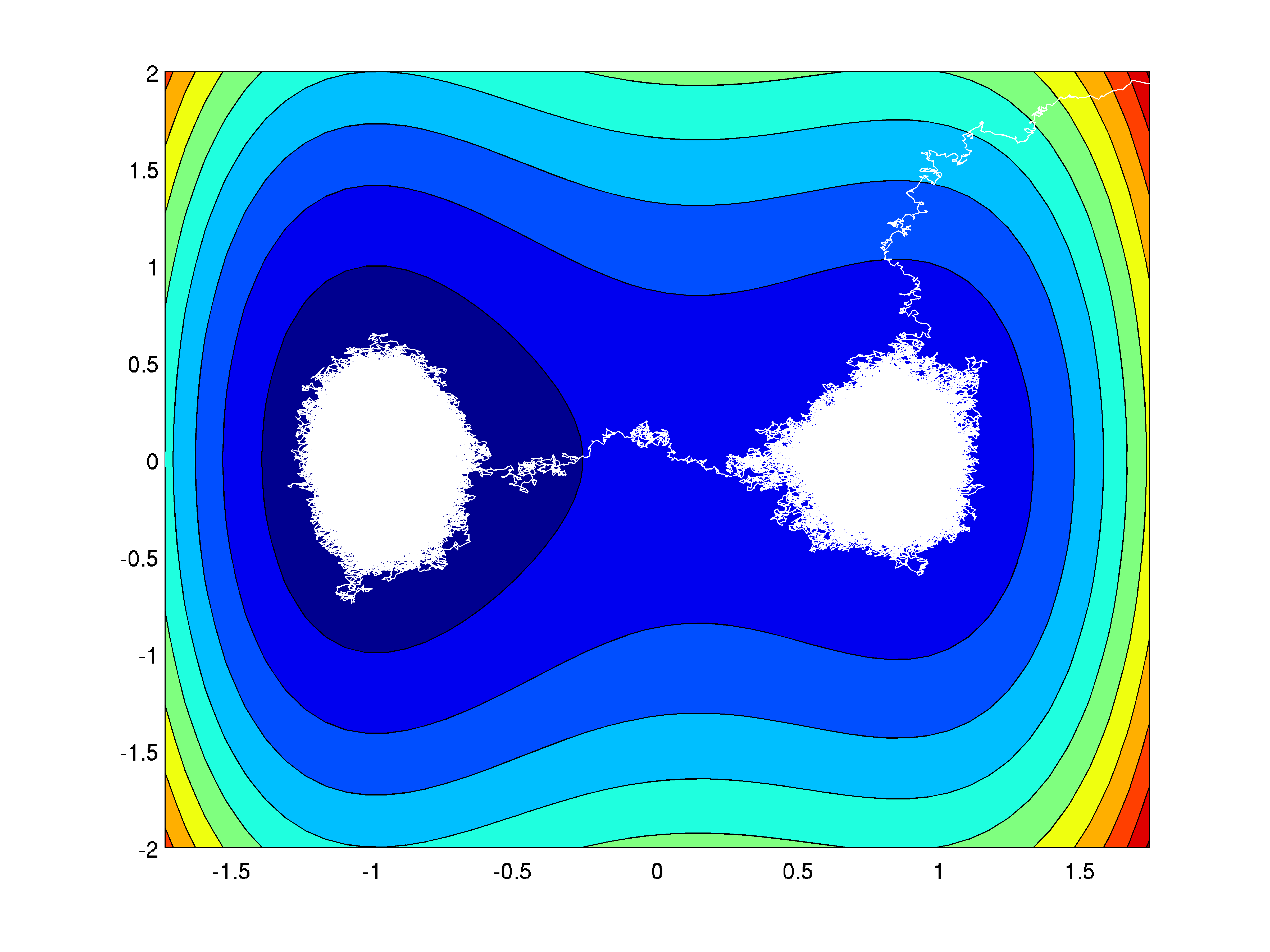
Sample path of a SDE in a double well potential

The trajectory shows a scale separation and spends a long time inside the individual basins of attraction for the local minima of $H$ (wrt. deterministic gradient flow $\dot x_t = -\nabla H(x_t)$ ) before doing a transition between the basins of attraction. The proof carries over this strategy by decomposing the measure $\mu$ roughly along the basin of attractions denoted by $\Omega_i$ with $i=1,\dots , M$ the number of local minima. Then $\mu$ has the mixture representation

\mu = Z_1 \mu_1 + \dots + Z_M \mu_M ,

where $\mu_i$ are the conditional probability measures with support in $\Omega_i$ and $Z_i = \mu(\Omega_i)$ . This decomposition carries over to a splitting of the variance and entropy as follows:

\operatorname{var}_\mu(f) = \sum_{i=1}^M Z_i \operatorname{var}_{\mu_i}(f) + \frac{1}{2} \sum_{i,j=1}^M Z_i Z_j \left( \int f d \mu_i - \int f d\mu_j \right)^2

and likewise for the entropy.

The local variances and entropies are estimated by constructing a Lyapunov function for the dynamics. For a background on the Lyapunov technique see (Patrick Cattiaux, Arnaud Guillin. Functional Inequalities via Lyapunov conditions. IF_ETE. 2010. <hal-00446104v2>). We slightly generalized the technique to cope with bounded domains by demanding appropriate Neumann boundary conditions for the Lyapunov function. Moreover, we succeeded also to construct a Lyapunov function, which made a fine analysis arond saddle points necessary.

The other part in the variance invoving the term $\left( \int f d \mu_i - \int f d\mu_j \right)^2$ was estimated using a Benamou-Brenier representation of the $H^{-1}(d\mu)$ , which we called a weighted transport distance. This cost representation allowed to construct a sufficiently flow of pushforwards connecting $\mu_i$ and $\mu_j$ .

Metastability in discrete setting

This ongoging project (with Martin Slowik) considers the discrete counterpart of the above dynamic, i.e. Markov chain on a discrete state space $S$ written with stochastic generator as

(Lf)(x) := \sum_{y\in S} p(x,y) (f(y) - f(x)) .

We assume the existence of a reversible invariant measure $\mu$ such that the detailed balance condition $\mu(x) p(x,y) = \mu(y) p(y,x)$ holds. The crucial idea from the continuous case to decompose the potential along the basin of attractions does not translate immediatley, since there is no canonical deterministic dyanmic associated with the generator $L$ , i.e. the role of $\varepsilon$ is hidden inside.

We characterize metastability following the potential theoretic approach (see A. Bovier and F. den Hollander: Metastability – a potential theoretic approch) as follows: The Markov process $\{ X(t) \}$ with generator $L$ is $\varrho$ -metastable with respect to metastable points $M$ , if

\frac{ \max_{m\in M} \mathbb{P}_m(\tau_{M\setminus m} < \tau_m) }{\min_{A\subset S \setminus M} \mathbb{P}_{\mu_A}(\tau_M < \tau_A )} \leq \varrho \ll 1 ,

where $\mu_A$ is the conditial measure on $A$ . Hereby, for a set $A \subset S$ , $\tau_A$ is the first hitting time if $X_0 \not\in A$ and else the first return time to $A$ .

For a metastable Markov chain, one can associate to each metastable point $m\in M$ its stochastic valleys in terms of hitting probabilities: The point $x$ belongs to the valley of $m$ if among the hitting probabilities to start in $x$ and to hit any $\tilde m \in M$ the largest one is attained for $m$ . This allows to carry over the decomposition idea from continuous state spaces.

Moreover, the above stochastic definition has an analytic connection via capacities by the identity

\operatorname{cap}(A,B) = \mu(A) \mathbb{P}_{\mu_A}( \tau_B < \tau_A ) .

The main question of the project was to show in generality that the above definition without any further model assumptions on the rates is already enough to prove Poincaré and logarithmic Sobolev inequalities with error bounds depending only on $\varrho$ and maybe on the cardinality of $M$ .

The program succeeded with the help of a robust capacitary inequality, which was established for Sobolev spaces by Vladimir Maz’ya (see V. Maz’ya. Sobolev Spaces: with Applications to Elliptic Partial Differential Equations and references therein for the history). We translated the inequality to discrete state spaces, where it reads:

Capacitary inequality

For $f: \mathbb{R} \to S$ define by $A_t \subset S$ its super-level sets $A_t := \{ |f| > t\}$ . Moreove, assume that $f|_B \equiv 0$ , then it holds

\int_0^\infty 2 t \operatorname{cap}(A_t , B) dt \leq 4 \mathcal{E}(f) ,

where $\mathcal{E}(f) := \langle f , (-Lf) \rangle_\mu$ is the Dirichlet-form associated to the generator $L$ .

Exploiting the consequences of the above inequality allows to conclude estimates of

C_{\mathrm{PI}}

and

C_{\mathrm{LSI}}

in terms of capacities with error bounds of the form

1+O(\sqrt{\varrho | M|})

. For furhter details see the proceedings and article:

A. Schlichting, M. Slowik: Capacitary inequalities in discrete setting and application to metastable Markov chains, Oberwolfach Report 35/2015. [ link | pdf ]
André Schlichting, Martin Slowik. Poincaré and logarithmic Sobolev constants for metastable Markov chains via capacitary inequalities. Accepted at Annals of Applied Probability [ arXiv | pdf ]